- You are expected to work in a team of two or three.
- Due: Friday August 1st at 11pm EDT (Baltimore time). Note: late submissions will not be accepted, please plan accordingly.
Learning Objectives
- Reading and writing file data
- Classes and objects
- Constructors, destructors, assignment operators, and the rule of 3
- Object-oriented design
- Operator overloading
- Trees (dynamic linked structures)
- Recursion
- Exceptions and exception handling
Overview
In this project, you will implement a program to render images based on plotting mathematical functions.
An example plot
Here is an example plot input file. (This is available as input/example04.txt in
the starter files.)
Plot 0 -2.5 40 2.5 640 480
Function fn1 ( sin x )
Function fn2 ( * 1.6 ( cos x ) )
Color fn1 100 100 255
Color fn2 100 255 100
FillBetween fn1 fn2 0.4 128 0 200
This plot produces the following image (click for full size):
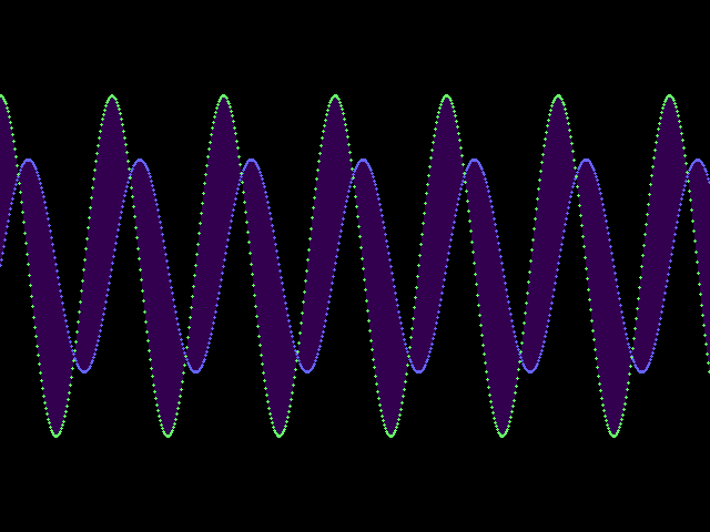
Here is a quick overview of the meaning of the example plot input file:
- The
Plotdirective indicates that the plot will show the region of the x/y coordinate plane where \(0 \le x \le 40\) and \(-2.5 \le y \le 2.5\), and the generated image will have the dimensions 640x480 - The first
Functiondirective indicates that the function calledfn1will plot the function \(y=\sin x\) - The second
Functiondirective indicates that the function calledfn2will plot the function \(y=1.6 (\cos x)\) - The first
Colordirective indicates that the plot offn1will use the color \((100,100,255)\) (colors are RGB triples, with color component values in the range 0–255) - The second
Colordirective indicates that the function calledfn2will use the color \((100,255,100)\) - The
FillBetweendirective indicates that the area betweenfn1andfn2should be filled with the color \((128,0,200)\) at an opacity of \(0.4\)
The detailed semantics of the various directives are described below.
Getting started
To get started on the project, use git clone to clone the final project
repository we have created for you. Also, use git pull to make sure that
your clone of the cs220-sp23-public repository is up to date.
Then, copy the starter files into your final project repository.
Assuming your current directory is your clone of your team’s final project
repository, you could use the following commands to copy the files:
cp -r ~/cs220-sp23-public/projects/final/* .
cp ~/cs220-sp23-public/projects/final/.gitignore .
Once you have copied the starter files, use git add, git commit,
and git push to incorporate them into your team’s repository.
Deliverables
There are three deliverables:
- The program code, along with a
READMEandgitlog.txt - A UML class diagram showing the important classes in the program and their relationships
- Completing the Final Project Contributions survey on Gradescope
One member of the team (and only one member!) should submit deliverables 1–2 to Gradescope in a zipfile. See the Submitting section. Be sure to add all of the group members to the submission on Gradescope.
Each team member will need to complete the final project contributions survey on Gradescope individually.
Detailed semantics
Compiling, program invocation
The Makefile should produce an executable called plot. As always,
we expect your code to compile without warnings with the compiler
options -std=c++14 -Wall -Wextra -pedantic. You can use the provided
Makefile, although if you want to write your own, or modify the
provided one, you can.
Note that the provided Makefile doesn’t have any explicit targets for
object (.o) files. These are generated by running the command
make depend
This works by having the compiler analyze the source files to determine
which header files each one depends on. Note that if you modify any
source or header files to add or remove #include directives, you
should run make depend again to regenerate the source and header
file dependencies.
The program is invoked as
./plot input_file output_file
The input_file argument specifies the input plot file.
The output_file argument is the PNG image file to write. (It should end
in the file extension .png.)
Plot files
A plot file is a series of directives. Each directive is specified on
one input line. There are 6 types of directives: Plot, Function, Color,
FillAbove, FillBelow, and FillBetween.
The items in a directive will be each be separated by at least one whitespace character. It is also possible that there could be leading or trailing whitespace characters in a directive.
The Plot directive has the following form:
Plot xmin ymin xmax ymax width height
The xmin, ymin, xmax, and ymax floating point values define the region of the x/y coordinate plane rendered by the plot. The width and height integer values specify the dimensions of the rendered image. Note that xmin must be less than xmax, and ymin must be less than ymax. Also, width and height must both be positive.
A plot input file must specify exactly one Plot directive.
The Function directive has the following form:
Function fn_name expression
fn_name is the name of the function, so that it can be referred to by
Color directives and the various Fill directives.
expression is a sequence of one or more tokens consistuing a prefix expression
which specifies the mathematical function to be plotted.
(See Functions and expressions below for details.)
The Color directive has the following form:
Color fn_name r g b
fn_name is the name of a function defined in a Function directive.
r, g, and b are the R/G/B color component values for the color
with which the function should be plotted.
The FillAbove directive has the following form:
FillAbove fn_name opacity r g b
fn_name is the name of a function defined in a Function directive.
opacity is a floating point value between 0.0 and 1.0 (inclusive)
specifying the opacity of the fill color.
r, g, and b are the R/G/B color component values for the fill color.
FillAbove indicates that the area above the function (where the \(y\) values
are greater than the value of the function) should be filled.
The FillBelow directive has the following form:
FillBelow fn_name opacity r g b
The values in a FillBelow directive have the same meaning as in a
FillAbove directive. FillBelow indicates that the area below the
function (where the \(y\) values are greater than the value of the function)
should be filled.
The FillBetween directive has the following form:
FillBetween fn_name1 fn_name2 opacity r g b
The values in a FillBetween directive have the same meaning as in
FillAbove and FillBelow directives, except there are two function names,
fn_name1 and fn_name2. FillBetween indicates that the area
beween the two functions, meaning where \(y\) is greater than one function
but less than the other, should be filled.
Functions and expressions
The mathematical functions specified by Function directives have the meaning
y=expr, where expr is a prefix expression.
Prefix expressions have one of the following forms:
xpi- a literal numeric (floating-point) value
(function_name arguments)
function_name is one of sin, cos, +, -, *, and /.
arguments is a sequence of 0 or more prefix expressions.
Because an expansion of arguments can include arbitrary (nested) prefix
expressions, prefix expressions are inherently recursive.
Prefix expressions are so-called because when a function is used, it
preceeds the argument values to which it is applied. The prefix expressions
in the plot program are similar to Lisp S-Expressions.
A critical idea to understand is that expressions can and should be represented
as a tree. Nodes representing
x, pi, or a literal numeric value are leaf nodes, meaning that they
have no child nodes. A node representing a function will have one child
node for each argument expression.
For example, consider the following prefix expression:
( + ( sin ( * 1.33 x ) ) ( * 0.25 ( cos ( * 6.7 x ) ) ) )
We could write this as an infix expression as something like \((\sin 1.33 x) + (0.25 (\cos 6.7 x))\). As a tree, this expression could be represented as

Note that every token in a prefix expression must be separated by at least one
whitespace character. This means that you can read the tokens in a prefix expression by
repeatedly extracting std::string values from the stream from which the expression
text is read.
The following pseudo-code explains how you could implement code to parse a prefix expression and build an expression tree from it.
// assume tokens is a sequence of tokens comprising
// the prefix expression
function parsePfxExpr(tokens) {
  n = remove first token from tokens

  if (n is "x", "pi", or a literal number) {
    create appropriate expression node and return it
  } else if (n is a left parenthesis) {
    n = remove first token from tokens

    if (n is none of sin, cos, +, -, *, or /) {
      throw exception // invalid function name
    }

    result = create appropriate function node

    while (first token of tokens is not right parenthesis) {
      arg = parsePfxExpr(tokens)
      add arg as child of result
    }

    remove first token from tokens // should be right paren

    return result
  } else {
    throw exception // unexpected token
  }
}
Since the algorithm repeatedly examines and removes the first token
from the sequence of tokens, you might consider using a std::deque
container to store the tokens, since it supports a pop_front() operation.
Note that the parsing algorithm described above allows any function to have any number (0 or more) of argument expressions. However, the following restrictions should be enforced:
sinandcosfunctions should have exactly one argument expression-and/functions should have exactly two argument expressions+and*functions may have any number (0 or more) of argument expressions
You don’t need to enforce these restrictions as part of parsing. It’s fine to check them later on.
Evaluating expressions
Evaluation is a recursive computation, starting from the root of the
expression tree. Different kinds of nodes will be evaluated differently.
For example, a node representing x will evaluate to the value of \(x\)
for which the expression is being evaluated. A node representing a
literal numeric value will evaluate to that value.
Nodes with children (arguments) will recursively evaluate their children
to compute their values. A node representing sin will evaluate to the
sine of its argument. A node representing + will evaluate to the
sum of its arguments.
You will notice tthat the Expr class in the starter code has a
member function
virtual double eval(double x) const = 0;
Each node type should be a class derived from Expr, and should
override the eval member function to perform the appropriate evaluation
strategy for that type of node.
The following table summarizes how each kind of node should be evaluated:
| Node type | Evaluation strategy |
|---|---|
x |
value of \(x\) |
pi |
value closest to \(\pi\) |
| literal number | the literal numeric value |
sin |
sine of argument |
cos |
cosine of argument |
+ |
sum of arguments (0 if there are no arguments) |
- |
difference of first and second arguments |
* |
product of arguments (1 if there are no arguments) |
/ |
quotient of dividing first argument by second |
Representing a plot
Before attempting to render a plot image, the program should build a complete representation of the plot directives as values and objects in memory. The plot bounds and dimensions, as well as the function, color, and fill directives should all be represented as data values and objects gathered in a central plot object.
Producing a rendered image
The rendered plot image should be created in memory as an Image object.
An Image is represented as an array of Color values, arranged in row-major
order with the top row of pixel colors first in the array.
Each pixel color should be black initially.
The renderer should first render the fills (FillAbove, FillBelow,
and FillBetween), in the order in which they appear in the plot input
file. To draw a fill, the renderer should consider every pixel in the
image. For each one, it should determine the \(x\) and \(y\) coordinates
the pixel represents. If a pixel’s coordinates are determined to be in
the fill area, then the pixel’s color should be adjusted based on the
fill’s opacity and color values. Say that the opacity value is \(p\).
The color component values of the updated pixel color should be changed
to \((1-p) \times c_{old} + p \times c_{new}\), where \(c_{old}\) is the original
color component value, and \(c_{new}\) is the fill color’s color component
value.
The renderer should then render the Functions, in the order in which they
appear in the plot file. For each function, the renderer should iterate over
the columns of the image, determine the \(x\) coordinate the column represents
(based on the bounds of the plot), and then determine the value of \(y\)
by evaluating the function for \(x\). The computed \(y\) value should be
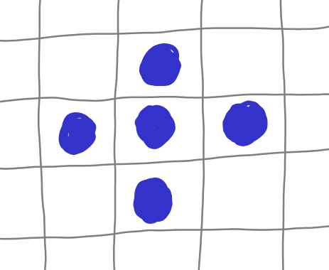
translated to a pixel row. The rendered should then draw 5 opaque pixels:
one at the appropriate pixel column and row based on the \(x\) and \(y\) values,
and four immediately above, below, left, and right of the center pixel.
In other words, a plotted point should be rendered like this (where
the blue dots represent a pixel to be draw for one plot point):
If a Color value for the function was specified, that color should be used
for the plotted pixels. Otherwise, white \((255,255,255)\) should be used.
Note that it is possible that some or all of the pixels for a particular point will be outside of the bounds of the image. The renderer should only draw the pixels that are within the bounds of the image.
In image data, the first row (row 0) is at the top of the image, and the row numbers increase going down, from the top of the image to the bottom. However, in the x/y coordinate plane, y values increase going up. You will need to take this into account when drawing pixels. The approach described in the following section (Pixel accuracy) explains how to do this.
Pixel accuracy
To ensure that your output image exactly matches the expected output image, please follow the recommendations in this section.
In the formulas shown below,
- \(x_{min}\) is the xmin value from the
Plotdirective - \(x_{max}\) is the xmax value from the
Plotdirective - \(y_{min}\) is the ymin value from the
Plotdirective - \(y_{max}\) is the ymax value from the
Plotdirective - \(w\) is the width value from the
Plotdirective (number of columns of pixels) - \(h\) is the height value from the
Plotdirective (number of rows of pixels) - \(f\) is a function (given a value \(x\), compute a corresponding value \(y\))
from the
Functiondirective specifying the function being plotted
In implementing code to perform these computations, be careful to
avoid integer division. Each computation involving a division
should be performed as a floating point division
(e.g., using double values.)
Fill operations. When rendering fill operations, each pixel represents a specific point in the x/y coordinate plane. For the pixel at row \(i\) and column \(j\), the corresponding point in the x/y plane is
\[(x_{j}, y_{i})\]where
\[x_{j} = x_{min} + (j/w) \times (x_{max}-x_{min})\]and
\[y_{i} = y_{min} + ((h-1-i)/h) \times (y_{max}-y_{min})\]By determining the precise x/y coordinates of a pixel, you can determine whether that point is above/below/between a function or functions, in order to determine whether or not the pixel should be colored as part of the fill.
Function plots. When rendering function plots, for each pixel column \(j\) in the image, your program should determine a corresponding pixel row \(i\) where the point should be plotted, and then color the pixel at that position, as well as the pixels above/below/left/right, using the color associated with the function. (Note that some or all of these pixel locations could be be outside the bounds of the image.)
For a pixel column \(j\), the pixel row \(i\) is computed as
\[i = h - 1 - \lfloor ((y - y_{min}) / (y_{max} - y_{min})) \times h \rfloor\]where
\[y = f(x_{min} + (j/w) \times (x_{max} - x_{min}))\]Note that your program should find the floor of a floating point value
by calling the floor function.
Color blending. When coloring a pixel for a fill operation, the resulting pixel color is blended from the original pixel color and the fill color, using the opacity value to determine the contributions of the components of the two colors being blended.
The color component values of the resulting color should be determined using the formula
\[c_{blend} = \lfloor (1 - \alpha) \times c_{orig} + \alpha \times c_{fill} \rfloor\]where
- \(c_{blend}\) is the blended color component value
- \(c_{orig}\) is the color component value of the original pixel
- \(c_{fill}\) is the color component value of the fill color
- \(\alpha\) is the opacity value
The computation should be done for each color component (red, green, blue) in order to fully determine the blended result color.
Design and implementation notes
The starter code provides a useful starting point for the program, and
illustrates how you could use classes and member functions to implement
the required functionality. There are a variety of TODO comments
indicating places where you will need to write code to implement
functionality, or places where you could add member functions, classes,
and other implementation code.
The main function (in main.cpp) can be largely used as-is. (Although,
you will need to implement exception handling.) It assumes that
your program will have a Reader class whose job is to read the
plot file and a Renderer class whose job is to render the plot into
a result Image object.
You are allowed to make any and all changes that your group decides on. It is completely up to you how to structure and implement your code. However, part of your grade will be based on design and coding style. As always, we expect that your code will be clean, readable, and will have appropriate comments to explain the code to the reader.
Here is a brief guide to the source code and classes that are provided in the starter code:
| Files | Class defined | Notes |
|---|---|---|
bounds.h/cpp |
Bounds |
represents the bounds of the plot |
color.h |
Color |
represents an RGB color value |
exception.h/cpp |
PlotException |
exception type thrown if a fatal error occurs |
expr.h/cpp |
Expr |
expression node type |
expr_parser.h/cpp |
ExprParser |
parses an expression and builds an expression tree |
fill.h/cpp |
Fill |
represents a fill directive |
func.h/cpp |
Function |
represents a function to be plotted |
image.h/cpp |
Image |
image data, can be written as a PNG file |
main.cpp |
n/a | main function: reads plot input, renders it to PNG |
plot.h/cpp |
Plot |
represents the plot directives (the plot object) |
reader.h/cpp |
Reader |
reads plot file to populate a Plot object |
renderer.h/cpp |
Renderer |
renders a Plot object to produce an Image |
Exception handling
When the program encounters a fatal error, it should throw a PlotException.
The main function should handle a PlotException by catching it, printing
an error message to std::cerr, and exiting the program with a non-zero return code.
The error message should be a single line of text of the following form:
Error: description of error
where description of error is the text returned by calling .what() on the exception
object.
The following are situations that should result in an exception being thrown and handled:
- invalid plot directives in plot input file, such as wrong
number of arguments to a directive, or invalid arguments to
a directive, for example
- invalid plot bound (e.g., xmin is not less than xmax)
- invalid image dimensions (e.g., width is not positive)
- the wrong number of arguments are passed to a function
(e.g.,
sinwith more than 1 argument) - error parsing prefix expression
- attempt to divide by 0
- unknown function name in expression
- error writing PNG file (
image.cppalready has code to detect these errors and throw an exception) - more than one
Colordirective for a function - fill directive referring to a nonexistent function name
The exact error message description your program produces for these errors is up to you.
Testing
As with the Midterm Project, you will need to have a way to view image files in your ugrad account.
The starter files include an input directory with example plot files,
and an expected directory with the expected outputs for each example
plot file. You can use the compare program to compare your program’s
output with the expected output.
For example, here is how you could test your program with the
input/example04.txt plot input file:
$ mkdir -p actual
$ ./plot input/example04.txt actual/example04.png
$ compare -metric RMSE actual/example04.png expected/example04.png \
  actual/example04_diff.png
$ echo $?
(Note that the compare command above is specified as being on two lines,
with the backslash \ used as a line continuation, but you could specify
all of the command line arguments on a single line.)
If the echo $? command outputs “0”, then your program’s image output
was identical to the expected output. Otherwise, the “diff” image file produced
by the compare program (in this case, actual/example04_diff.png)
will have red pixels wherever your program’s output differed from
the expected output image. Note that we expect your program’s output
to match the expected output exactly: see the Pixel accuracy
section above.
Make sure that you use valgrind frequently to test your program to ensure that there
are no memory errors or memory leaks.
Development strategy
Roughly, your main development goals should be
- reading the plot input and building a
Plotobject to represent it, and - rendering a plot to an
Image
The first goal is the responsibility of the Reader object, and the second
is the responsibility of the Renderer object.
The problem of parsing expressions to build an expression tree is a component of goal #1, but is a well-defined task in its own right, so you could work on it independently of other parts of the progrm.
As with all larger and more complex programs, try to make progress in small increments, carefully testing your code with each step. Commit and push your changes each time you implement and test additional functionality. Make sure you create meaningful commit messages.
A good way to get started is to add empty "stub" versions of all of
the member functions which are required to get the plot
program to compile. Once that's done, you can start implementing the
program functionality.
UML Diagram
Once you have implemented all of the classes in the program, your group should create a UML class diagram showing the relationships between the classes.
We recommend using a vector drawing program for your diagram. yEd is a good free “graph editor” which can produce reasonable UML diagrams. However, you can use any program that can produce a PDF file.
Your UML diagram should be exported to a PDF file called UMLDiagram.pdf.
Make sure that your diagram uses the correct notation for each kind of relationship. The most important ones are:
Generalization, a.k.a. “Is-A”, a.k.a. “Inheritance”:

Aggregation, a.k.a. “Has-A”:

Note that “has-a” relationships are typically used in cases where one object contains (by reference or by value) one or more instances of another kind of object.
Association, a.k.a. “Uses”:

Note that association relationships are typically used for situations where an object uses an instance of another class to carry out some of its behavior, but does not have an “ownership” relationship with that object.
Your diagram does not need to indicate class members such as member variables and member functions. However, adding one or two of the most important public member functions can be a nice way to indicate the functionality of each class.
Submitting
Before you submit, make sure each of the source and header files has a comment at the top of the file indicating the names and JHED IDs of each team member.
Your submission zipfile must contain a README, gitlog.txt, Makefile,
UMLDiagram.pdf, and all source and header files needed to compile the program.
A command to create the submission zipfile might look like this:
zip -9r submission.zip *.h *.c *.cpp Makefile README gitlog.txt UMLDiagram.pdf
Your README must include:
- A section titled ‘TEAM’ which lists each team participant’s name and JHED id
- A section titled ‘DESIGN’ which gives a brief explanation of overall design
- A section titled ‘COMPLETENESS’ which indicates how complete your solution is (i.e. are you aware of any missing/incorrect functionality?).
- An optional section titled ‘SPECIAL INSTRUCTIONS’ which indicates how we should run your code. (Hopefully this is not necessary — if it is, you may lose points per the requirements above.)
- An optional section titled ‘OTHER’ which gives the graders any additional information you want the graders to know about your submission.
One member of your team should submit the zipfile to the Final Project assignment on Gradescope. Make sure that all team members are added to the submission.
Don’t forget that each team member must also submit the Final Project Contributions survey on Gradescope.